
Invariance and Learning Fair Representation
Learning fair representation
Machine learning algorithms often treated sub-population unfavorably, e.g., predicting the likelihood of crime on the grounds of ethnicity, gender or age. The algorithmic fairness is then proposed to mitigate the prediction bias for the protected feature such as gender and age.
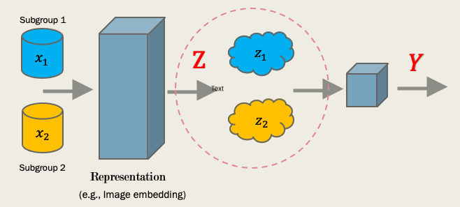
Specifically, we are interested in learning a fair representation which can easily transfer the unbiased prior knowledge to the downstream tasks. E.g, in language understanding, the fair embedding provides both useful and unbiased representation for different objectives such as translation or recommendation.
Invariance and Fair Representation
Intuitively, if we could learn invariant prediction behaviors on different subgroups of population, we could achieve certain kinds of fairness. As the invariance suggests some identical statistical properties for different subgroups such that the prediction discrimination could be alleviated.
Formally, we denote the input as \(X\), ground truth output as \(Y\), sensitive attribute as \(A\) (such as age) and the representation function \(\lambda: X \to Z\) that maps the input into a latent variable \(Z\). Then based on different fair definitions, we have three popular definitions:
Independence Rule (or Demographic Parity) \(A \perp \!\!\! \perp Z\). It learns a representation \(\lambda(X)\) such that the embedding variable is independent to the sensitive attribute \(A\). E.g, consider predict the health risk of patients, it ensures that the latent space have the identical distribution under different subgroups \(P(Z|A=a)=P(Z|A=a’)\).
Separation Rule \(A \perp \!\!\! \perp Z | Y\). It enforces a stronger constraint by encouraging the conditional independence w.r.t. the label \(Y\). E.g, health risk system ensures that the latent space have the identical distribution under different subgroups for the high risk group \(P(Z|A=a,Y=\text{high})=P(Z|A=a’,Y=\text{high})\).
Sufficiency Rule \(A \perp \!\!\! \perp Y | Z\). It ensures the same expected conditional output. E.g, if two patients from two subgroups have the same latent observation \(Z=s\), their expected true output should be identical: \(P(Y|Z=z,A=a)=P(Y|Z=z,A=a’)\).
Why sufficiency? The fundamental limitations of Independence and Separation lie in the inherent trade-off of fair and informative predictions: encouraging the fairness could induce the degradation of the prediction performance (even we have the data generation distribution!). Thus we will focus on the learning fair representation w.r.t. sufficiency rule, which could possibly achieve these objectives simultaneously.
Learning fair representation w.r.t. sufficiency rule
In our paper, we consider a fair representation learning approach to achieve the sufficiency rule. The intuition is depicted as: if the optimal predictors \(h^{\star}: Z \to Y\) are invariant for each subgroup \(A=a\). The corresponding representation \(\lambda(X)\) is fair w.r.t the sufficiency.
In plain language, suppose we have two subgroups \(A=\{0,1\}\) and a fix representation \(Z=\lambda(X)\), then we train two predictors \(h\) for each subgroup w.r.t some prediction loss, if the optimal predictor are invariant \(h^{\star}_{0} = h^{\star}_{1}\), then \(\lambda\) satisfy the sufficiency rule (see Fig(a)).
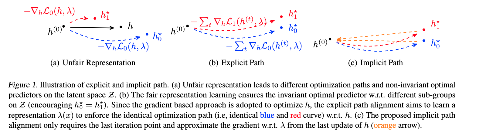
The aforementioned intuition can be naturally formulated as a bi-level optimization, where we need to adjust the representation \(\lambda\) (in the outer-loop) to satisfy the invariant optimal predictor \(h\) (in the inner-loop).
In deep learning, if we further adopt the gradient-based approach in solving this bi-level objective, a straightforward solution is to learn the representation \(\lambda\) to fulfill the identical explicit gradient-descent directions in learning optimal predictor \(h^{\star}\) of different groups, shown in Fig.(b). Clearly, if the inner gradient descent step of each sub-group is well-aligned, their final predictors (as the approximation of \(h^{\star}\)) will be surely invariant. However, the corresponding algorithmic realization is challenge in the deep learning regim:
It requires storing the whole gradient steps, which induces a high memory burden;
the embedding function \(\lambda\) is optimized via backpropagation from the whole gradient optimization path, which induces a high computational complexity.
Thus in this paper, we propose an implicit path alignment, shown in Fig.(c). Namely, we only consider the final (\(t\)-th) update of the predictor \(h^{(t)}\), then we update representation function \(\lambda\) by approximating its gradient at point \(h^{(t)}\) through the implicit function. By using the gradient approximation, we do not need to store the whole gradient steps and conduct the backpropagation through the entire optimization path.
It is worth mentioning that the idea shares several similarities with the recent proposed IRM (Invariant Risk Minimization), where the objective is also to achieve sufficient representation: \(P(Y|Z,A=a) = P(Y|Z,A=a’)\). (Though the practical approximation IRM_V1 or its variant seems not capturing the true invariance, due to the optimization difficulties.)
Formulation and gradient approximation
Assume \(\mathcal{L}\) is the prediction loss, the intuition could be formulated as:
\[ \min_{\lambda} \mathcal{L}_0(h_0^{\star},\lambda) + \mathcal{L}_1(h_1^{\star},\lambda) \\ \text{s.t.} h_{0}^{\star} = h_{1}^{\star}, h_{0}^{\star} \in \underset{h}{\text{argmin}} \mathcal{L}_0(h,\lambda), h_{1}^{\star} \in \underset{h}{\text{argmin}} \mathcal{L}_1(h,\lambda). \]
If we adopt the Lagrangian approximation with fair constraint \(\kappa>0\), we have:
\[ \min_{\lambda} \mathcal{L}_0(h_0^{\star},\lambda) + \mathcal{L}_1(h_1^{\star},\lambda) + \kappa \|h_{0}^{\star} - h_{1}^{\star} \|^2 \\ \text{s.t.} h_{0}^{\star} \in \underset{h}{\text{argmin}} \mathcal{L}_0(h,\lambda), h_{1}^{\star} \in \underset{h}{\text{argmin}} \mathcal{L}_1(h,\lambda) \]
Thus the key is to estimate the gradient of \(\lambda\) in the auto-diff. Based on the chain rule, we need to estimate \(\nabla_{\lambda} h_0^{\star}\) (the response function). Note \(h_{0}^{\star} \in \underset{h}{\text{argmin}} \mathcal{L}_0(h,\lambda)\), then we have:
\[ \nabla_{h_0} \mathcal{L}_0(h_{0}^{\star},\lambda) = 0 \]
Then taking the total derivative w.r.t. \(\lambda\), we have:
\[ \nabla_{\lambda} h_0^{\star} = -\left(\nabla^2_{h_0} \mathcal{L}_0(h_0^{*}, \lambda) \right)^{-1} \left(\nabla_{\lambda}\nabla_{h_0}\mathcal{L}_0(h_0^{*}, \lambda) \right) \]
Then plugging in \(h_0^{\star} \approx h_0^{(T)}\), the last step of the gradient update, we could efficiently approximate the response function (along with other computational tricks).
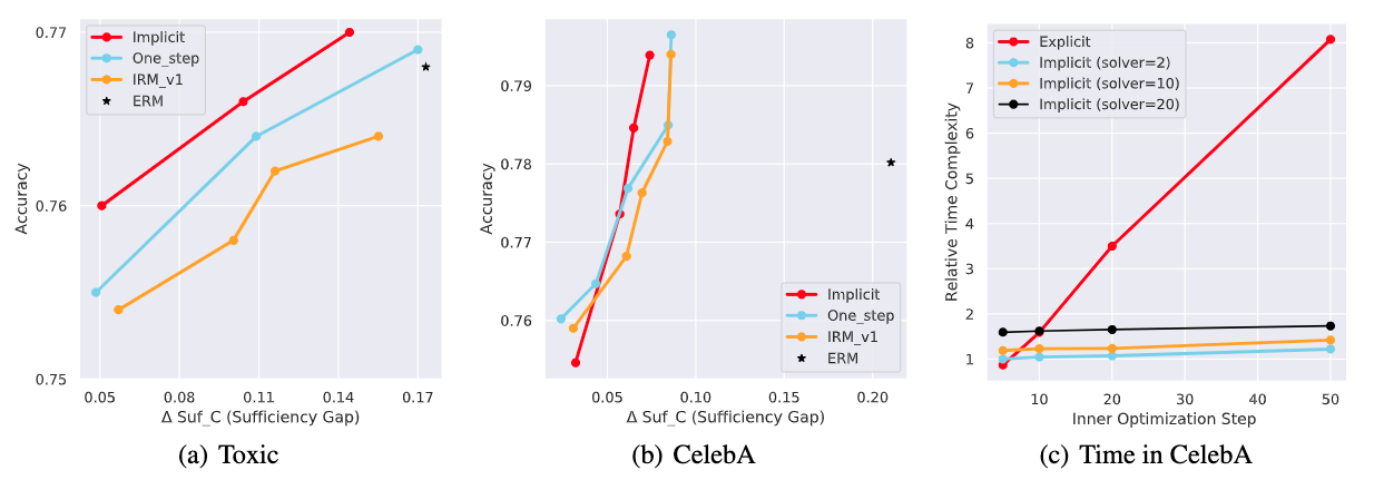
Empirical validations
We further show empirical benefits of proposed approach in two classification tasks (a) Toxic (b) CelebA, which demonstrated a consistent better accuracy-fair trade-off. We further demonstrate the computational benefits of proposed implicit gradient approximation (c), which remains stable under high inner-loop steps.
Summary
We consider a fair representation learning perspective to ensure the sufficiency rule. We naturally formulate the problem as a bi-level optimization and adopt implicit approximation to efficiently estimate the gradient.
CC BY-SA 4.0
C.Shui, Jun, 2022